Limit Order Book dimension reduction and clustering
Published:
Dimension Reduction for Limit Order Book Data and Applying SOM Clustering
Authors: Alireza Bakhtiari
An approach to dimension reduction for Limit Order book data and clustering
Limit-Order book data has been an interest to research for years now. It represents the dynamics of supply and demand in an online market. Therefore, it could be used in many different usages, including algorithmic-trading. In this work, I tried to propose a new way for reducing the size of this data structure. Moreover, I showed how these transformed data points could be clustered using the SOM algorithm.
Table of Contents
What is Limit Order Book?
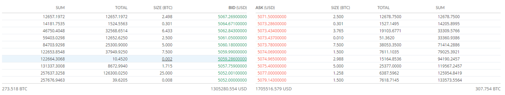
A limit order book is a record of outstanding limit orders maintained by the security specialist who works at the exchange. A limit order is a type of order to buy or sell a security at a specific price or better. ”Buy,” or ”bid” orders represent an intention to buy a certain amount of a security at some maximum price while ”sell” or ”ask” orders represent an intention to sell a certain amount of a security at some minimum price. The exchange is done by matching orders by price from the order book into a trade transaction between buyers and sellers.
Visualization
The most popular visualizations for the limit order book are as below: 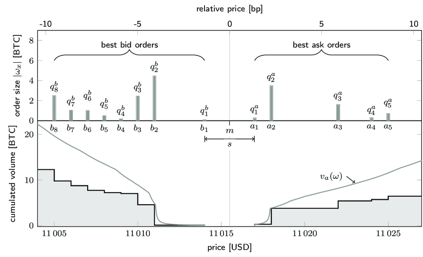
At the top is the normal representation, in which at each price tick is a volume indicating the amount of existing security in that exact price.
However, most of the time, the order book is visualized as below in online exchanges. In this representation, the cumulated amount of the security until that exact price is noted. This is a useful representation because a seller or a buyer could see the number of available stocks(or currency) with higher(lower) than a price to sell(buy).
Visualization
The evolution of limit order book could be visualized in the latter visualization as follows:
This visualization represents the changes that happened in a limit order book of a security. The evolution of order book could indicate different situations in a financial market, including buy pressure, sell pressure, depth of the market, the volatility of price, etc. Therefore, the study of this evolution is important for many reasons.
Data
I use the data of the Ethereum market from year 2019, and snapshots are taken with a period of 1 minute. At each snapshot of the order book, we have 200 price ticks (100 asks and 100 bids) and their corresponding volumes, which indicates how much volume is available for less or more than this price point to buy or sell, respectively. Therefore, each snapshot could be stored as a 3-dimensional vector as follows, the first dimension indicates whether we are on the bid side or ask side, the second dimension specifies the volume or the price value, and the third dimension indicates the number of price/volume tick. 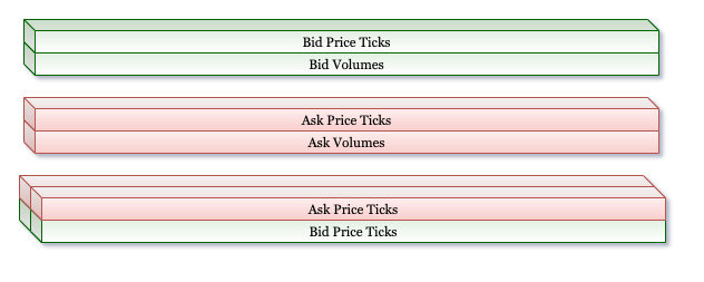 In result we will have a 4 dimension array of order book snapshots through time in one minute intervals.
Dimension Reduction
Each of our samples(3-dimensional order books) has 200 data points. This representation will not result in good clusters because of two reasons. First, SOM clustering is a distance-based method that could result poorly in very high dimensional spaces. Second, order books are stored in a cumulated fashion, so a single change in one price tick could result in a whole another order book as it affects subsequent ticks. Therefore, we need a more robust representation of them in order to get good clusters at the end.
Calcualte Price Buckets
We will start with the raw data of the order books in the 4-dimensional representation given above. I have 54000 snapshots of order books in my dataset.
print(raw_books.shape)
# output
(540000, 2, 2, 100)
We want to reduce the dimension of these raw order books at the end of the process. In this approach, we will specify some decimal numbers as cut-points. These numbers will be used on each sample (order book snapshot) individually, reducing their dimension from 200 to the desired number.
First, we extract the mid-price of each snapshot. Mid-price is the mean of the best ask price and the best bid price.
mid_prices = np.copy((raw_books[:, 1, 0, 0] + raw_books[:, 0, 0, 0]) /2)
print(mid_prices.shape)
# output
(540000,)
Mid-price is important in the study of order book shapes because the tick sizes are static (usually 0.01 dollar), but mid-price changes through time. For instance, first, consider mid-price of 100$. And the bid order at 100 tick from the mid-price 99.00$. In this case, the buyer is proposing a price with 99% of the actual mid-price. In another case consider the mid-price of 200$ and the bid order at the same point (100 tick in bid side) with a price of 199.00%. This time the bid price is 99.5% of the mid-price. It is worth noting that these two scenarios are different as buyers offer different price ratios to the actual mid-price. Therefore, in order to resolve this problem, we have to divide each tick’s actual price (mid_price + number_of_tick * 0.01$) to the mid-price in that snapshot. Therefore, in order to resolve this problem we have to divide each tick’s actual price (mid_price + number_of_tick * 0.01\$) to the mid-price in that snapshot.
price_ticks = raw_books[:, :, 0, :] / mid_prices[:, np.newaxis, np.newaxis]
print(price_ticks.shape)
(540000, 2, 100)
Then we extract the volumes on each price tick as follows:
price_volumes = raw_books[:, :, 1, :]
print(price_volumes.shape)
(540000, 2, 100)
Now we use np.histogram to divide volumes according to their prices into equal-sized buckets(bins value is hyper-parameter but does not have a strong effect on the result). Because of the different distribution in ask and bid sides, we have to separate their histograms.
bins = 100 * 1000
bid_hist, bid_bin_edge = np.histogram(price_ticks[:, 0, :],
                                      weights=price_volumes[:, 0, :],
                                      bins=bins)
ask_hist, ask_bin_edge = np.histogram(price_ticks[:, 1, :],
                                      weights=price_volumes[:, 1, :],
                                      bins=bins)
print(bid_hist.shape, bid_bin_edge.shape)
print(ask_hist.shape, ask_bin_edge.shape)
(100000,) (100001,)
(100000,) (100001,)
Now, we use np.cumsum to sum over the volumes of the price histograms. By doing so, in each bucket, we have the amount of volume prior to that. Further, we divide these volumes to their max in order to achieve the CDF of volumes according to their prices.
bid_cumulated_volumes = np.cumsum(bid_hist)
ask_cumulated_volumes = np.cumsum(ask_hist)

bid_volume_cdf = bid_cumulated_volumes / bid_cumulated_volumes[-1]
ask_volume_cdf = ask_cumulated_volumes / ask_cumulated_volumes[-1]

print(bid_volume_cdf.shape)
print(ask_volume_cdf.shape)
(100000,)
(100000,)
At this point, we will specify some decimal numbers, each of which indicates a price-ratio used for bucketing order books. But, first, we have to specify the number of desired buckets (this will be the number of dimensions in the end)
TARTGET_DIMENSION = 25
In the following function we will extract bucket_edges
def calculate_buckets_edge(price_volume_cdf, bid_edges):
    buckets_edge = []
    current_bucket = 1
    for i in range(1, bins):
        if price_volume_cdf[i] >= (1 / TARTGET_DIMENSION) * current_bucket:
            buckets_edge.append(bid_edges[i])
            current_bucket += 1
    return buckets_edge

bid_buckets_edge = calculate_buckets(bid_volume_cdf, bid_bin_edge)
ask_buckets_edge = calculate_buckets(ask_volume_cdf, ask_bin_edge)

print([f'{edge:.4f}' for edge in bid_buckets_edge])
print([f'{edge:.4f}' for edge in ask_buckets_edge])
['0.9908', '0.9920', '0.9927', '0.9932', '0.9936', '0.9941', '0.9945', '0.9949', '0.9953', '0.9958', '0.9962', '0.9966', '0.9971', '0.9974', '0.9977', '0.9979', '0.9981', '0.9983', '0.9985', '0.9987', '0.9989', '0.9991', '0.9993', '0.9995', '1.0000']
['1.0005', '1.0007', '1.0008', '1.0010', '1.0012', '1.0014', '1.0016', '1.0018', '1.0020', '1.0022', '1.0024', '1.0027', '1.0030', '1.0035', '1.0039', '1.0044', '1.0048', '1.0053', '1.0057', '1.0062', '1.0067', '1.0073', '1.0080', '1.0094', '1.0959']
These numbers specify ratios that specify at which points each order book has to be cut on its price ticks. These numbers are lower than one for the bid side because the bid prices are always less than mid-price. While, on the ask side, these cut points are slightly bigger than one as ask prices are always greater than mid-price in each snapshot.
Finally, we apply these cut points on each of our samples as follows:
def apply_buckets_on_order_book(order_book):
    bid_prices = order_book[0, 0, :]
    ask_prices = order_book[1, 0, :]

    mid_price = (bid_prices[0] + ask_prices[0]) / 2

    # divide each tick price to mid price at that snapshot
    bid_prices /= mid_price
    ask_prices /= mid_price

    # Create a new array for transformed order book
    bids = np.zeros((TARTGET_DIMENSION, ), dtype=np.float32)
    bid_indices = np.searchsorted(bid_buckets, bid_prices)
    for i, index in enumerate(bid_indices):
        bids[index] += book[0, 1, i]

    bids = np.cumsum(bids)

    # Create a new array for transformed order book
    asks = np.zeros((TARTGET_DIMENSION, ), dtype=np.float32)
    ask_indices = np.searchsorted(ask_buckets, ask_prices)
    for i, index in enumerate(ask_indices):
        asks[index] += book[1, 1, i]

    asks = np.cumsum(asks)
    return np.concatenate([bids[::-1], asks])
Self-Organizing Map
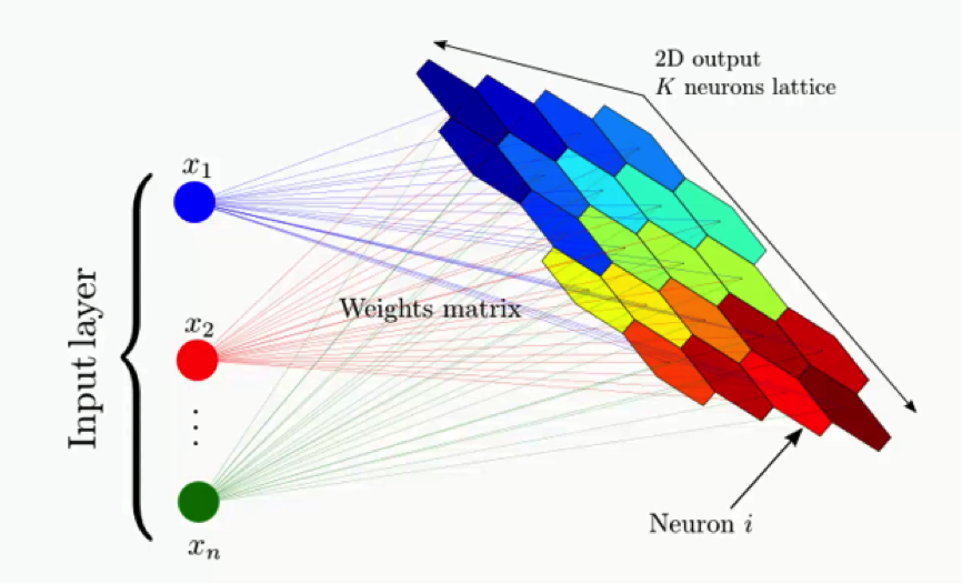
A self-organizing map (SOM) or Kohonen’s maps is a type of artificial neural network (ANN) that is trained using unsupervised learning to produce a low-dimensional (typically two-dimensional), discretized representation of the input space of the training samples, called a map, and is therefore a method to do dimensionality reduction. Self-organizing maps differ from other artificial neural networks as they apply competitive learning as opposed to error-correction learning (such as backpropagation with gradient descent), and in the sense that they use a neighborhood function to preserve the topological properties of the input space.
Architecture
SOM is formed from two layers, one is the input layer and the other one is the lattice. The lattice is a network of neurons connected to each other in specific architecture (e.g. hexogans, cubic, rectangular). Each of the neurons in an SOM gets the inputs point and calculates its distance from it as follows:
Training
Training could be seperated to three phases:
- Competetion
- Self update
- Neighbor update
All of the phases are applied to each input sample in order. In the competetion phase, the closest neuron to the input will win and the input will be assigned to it. Next, the winner neuron’s weight vector gets updated according to the input sample. In the end, each of the neighbors get updated related to their proximity to the winner. You can read detailed algorithm in this Link.
Apply SOM on Data
I use MiniSOM implementation of SOM as follows:
A = 7
B = 8
sigma = 1.1
learning_rate = .4
epoch = 80000
neighborhood_function = "gaussian"

from minisom import MiniSom

# Initialization and training
som = MiniSom(A, B, 2 * (TARTGET_DIMENSION + 1), sigma=sigma, learning_rate=learning_rate, activation_distance='euclidean',
              topology='hexagonal', neighborhood_function=neighborhood_function, random_seed=10)

som.train(price_bucket_books_vstack, epoch, verbose=True)
[ 80000 / 80000 ] 100% - 0:00:00 left
Result visualization:
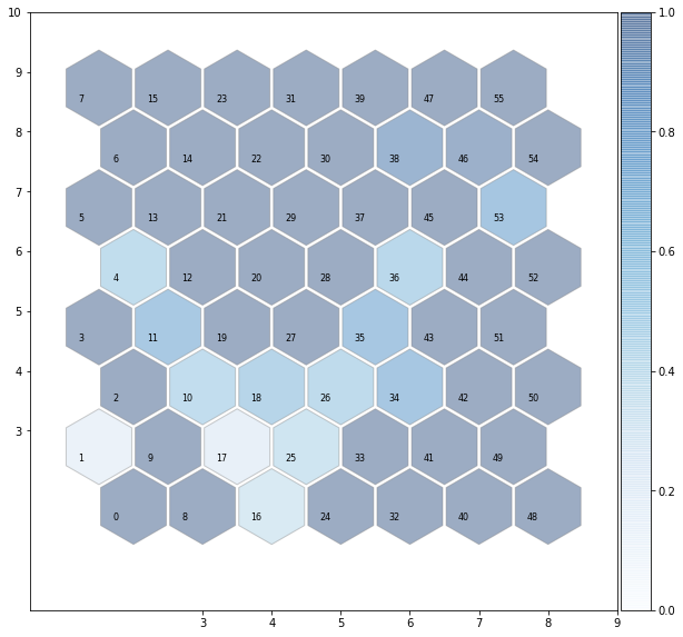
Now we can go ahead and see sum result of our clusters. We will select some samples from some clusters randomly and see the results.
winners = [ [] for i in range(weights.shape[0] * weights.shape[1]) ]
for cnt, x in tqdm(enumerate(price_bucket_books_vstack)):
    winner = som.winner(x)
    winners[winner[0] * weights.shape[1] + winner[1]].append(x)
import random

cluster_number = <cluster number>

neuron = winners[culster number]
print(len(neuron))
for book in random.choices(neuron, k=6):
    plt.bar(range(len(book)), book, label='Bars1', color='c')
    plt.show()
![]()
![]()
![]()